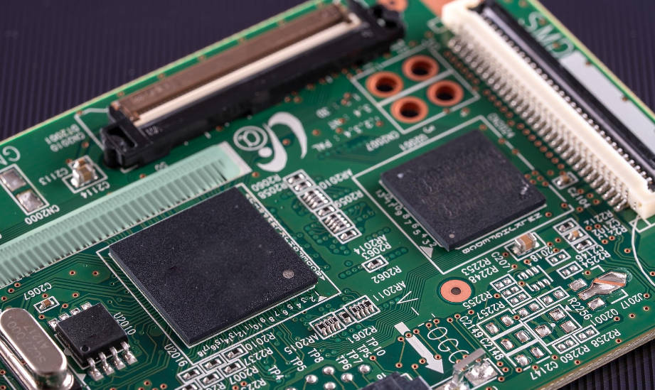
A printed circuit board does not become a high speed PCB simply because its operating clock runs at hundreds of megahertz or gigahertz. In hardware engineering, a board enters the high-speed regime the moment a signal’s edge transition time — its rise time (Tr) or fall time (Tf) — is fast enough relative to the trace length that the electrical trace stops behaving like an ideal lumped conductor and begins behaving like a distributed transmission line.
Evaluating whether a layout requires high-speed engineering rules comes down to two physical parameters: the driver switching speed and the physical propagation delay along the copper trace. When the signal transition is faster than the round-trip or fraction of single-trip propagation delay across the trace, unmanaged parasitics trigger signal distortion, ringing, electromagnetic interference (EMI), and false switching.
This guide breaks down the physical mechanism of signal rise time, establishes the quantitative critical trace length rule, details the design challenges that appear once this boundary is crossed, and highlights essential material and fabrication considerations for reliable production. If any of the vocabulary here is new to you, keep our high-speed PCB terminology glossary open alongside this page.

Frequency vs. Edge Rate: Why Traditional PCB Rules Fail Modern Circuits
A widespread misconception among hardware developers is equating high-speed operation strictly with clock repetition rate. A 10 MHz microcontroller clock driving an external bus might seem low-speed at first glance. However, if the output buffer driving that 10 MHz square wave transitions from logic 0 to logic 1 in 800 picoseconds, the spectral content generated by that rapid edge transition contains frequencies extending deep into the gigahertz range.
Modern sub-micron silicon processes, advanced FPGAs, and high-efficiency power semiconductors (such as GaN and SiC switches) deliver extremely steep slew rates by design to minimize internal switching losses and meet fast bus timings. Even if your system throughput or clock rate is modest, the fast voltage transition (dV/dt) and current surge (dI/dt) excite parasitic trace inductance and stray capacitance. If a layout relies on basic DC-continuity routing rules, these steep edge rates cause severe signal integrity issues, such as reflections from impedance discontinuities, ground bounce, and severe near-end crosstalk. The edge rate, not the clock rate, is what decides whether your layout needs transmission line rules — a distinction we unpack further in Rise Time vs. Clock Frequency.
What Is Signal Rise Time and How Does It Define Bandwidth?
Signal rise time is the duration required for a digital voltage pulse to transition between specified logic thresholds, typically measured from 10% to 90% (or 20% to 80%) of the steady-state logic swing.
The edge rate of this transition dictates the spectral energy of the signal. In frequency-domain analysis, the highest frequency component that dictates layout behavior is characterized as the “knee frequency” (Fknee). Below Fknee, the energy content of the signal spectrum rolls off at a rate of 20 dB/decade; above Fknee, the roll-off steepens to 40 dB/decade.
Using Dr. Howard Johnson’s established formulation, the effective spectral bandwidth is calculated as:
(Note: In linear ramp approximations, 0.35 / Tr is frequently referenced; the 0.5 factor accounts for practical, steeper Gaussian transition profiles.)
| Rise Time (Tr) | Equivalent Bandwidth (Fknee) | Design Implication |
|---|---|---|
| 10.0 ns | 50 MHz | Lumped circuit rules often suffice |
| 2.0 ns | 250 MHz | Transmission line effects emerge |
| 1.0 ns | 500 MHz | Impedance control mandatory for traces > 2 inches |
| 0.5 ns (500 ps) | 1.0 GHz | Strict return path continuity and loss control required |
| 0.1 ns (100 ps) | 5.0 GHz | Dielectric absorption and copper skin effect dominate |
As the table demonstrates, a sub-nanosecond rise time introduces multi-gigahertz spectral energy into the copper interconnect. At these harmonic levels, standard FR-4 dielectric losses and copper surface roughness begin attenuating the signal, rounding off the edges and degrading timing margins.
The Critical Trace Length Rule: When Does a Trace Become a Transmission Line?
To determine whether an individual trace must be routed and manufactured as a transmission line, engineers compare the signal propagation delay (Td) to the signal rise time (Tr).
In typical PCB substrates such as standard FR-4 (with an effective relative dielectric constant εr ≈ 4.0 to 4.5), signals propagate along copper traces at roughly 6 inches per nanosecond (approximately 150 to 180 picoseconds per inch for microstrip layers, and roughly 170 to 200 picoseconds per inch for stripline layers).
A widely adopted engineering threshold is the One-Sixth Rule (and under stricter noise margins, the One-Tenth Rule). A trace must be modeled as a transmission line with controlled characteristic impedance if the one-way propagation delay along its physical length exceeds one-sixth of the driver’s rise time:
Expressed in physical length (Lcrit):
(Where D represents the propagation delay per unit length, typically ~160 ps/inch for surface microstrips.)
Engineering Decision Workflow
- Extract Driver Rise Time: Identify the fastest specified transition time (Tr) from the component’s IBIS model or datasheet (do not rely on typical values; use minimum/fastest edge rates).
- Calculate Signal Velocity: Determine the phase velocity based on the layer substrate’s effective dielectric constant (εeff).
- Determine Critical Length: Apply the Tr / 6 boundary. For example, if Tr = 1 ns, the critical threshold is roughly 1 inch (25.4 mm). Any interconnect exceeding 1 inch must be treated as a transmission line.
- Define Routing Strategy: If trace length exceeds Lcrit, implement matched characteristic impedance routing, controlled termination, and continuous reference planes.
When trace geometries exceed this critical length without matched termination, reflected waves do not settle before the logic state transitions, resulting in signal overshoot, undershoot, and ring-induced double-triggering.
What Changes When Your Board Crosses the High-Speed Threshold?
Once interconnects exceed the critical trace length threshold, standard schematic-driven routing rules are no longer sufficient. Physical geometry directly dictates circuit behavior.
| Layout Attribute | Standard PCB Routing | High-Speed PCB Routing |
|---|---|---|
| Trace Impedance | Uncontrolled trace widths | Controlled impedance (e.g., 50 Ω single-ended, 100 Ω differential) |
| Signal Topologies | Stubs, branches, and daisy-chains | Point-to-point routing with matched termination |
| Return Path Routing | Ground fills where convenient | Continuous reference planes directly beneath traces |
| Reference Transitions | Vias placed freely | Ground return stitching vias placed adjacent to layer shifts |
| Length Matching | Unconstrained routing length | Strict skew and phase matching (within mils or picoseconds) |
| Via Geometries | Standard through-hole vias | Stub-minimized, backdrilled, or microvia structures |
Critical High-Speed Routing Rules
- Continuous Return Current Paths: High-speed return currents follow the path of least inductance directly underneath the signal trace on the adjacent reference plane, not the path of least DC resistance. Crossing plane splits, voids, or antipads introduces high loop inductance, creating signal distortion and radiated EMI. The discipline of keeping that path unbroken is covered in return path continuity across reference plane voids and splits.
- Controlled Termination Schemes: When traces function as transmission lines, source-series termination (Rs) or parallel end-termination must be added to absorb reflections and match the line’s characteristic impedance (Z0).
- Mitigating Discontinuities and Stubs: Every via acts as an LC network. On signals with sub-nanosecond rise times, the unused barrel of a through-hole via — the via stub — creates a quarter-wave resonant notch filter, causing signal attenuation at specific harmonic frequencies.
For designs requiring precision layer transitions and verified signal integrity, selecting appropriate high-speed PCB manufacturing services ensures that nominal track geometries translate to accurate physical impedance on the fabricated board. Where the transition density is high, HDI and ELIC build-ups let you replace long through-hole barrels with microvias instead.
Manufacturing High-Speed Boards: Materials, Tolerances, and Stackup Integrity
Designing a high-speed layout on CAD software is only half the battle; the bare board manufacturing process must hold tight physical and material tolerances to preserve signal fidelity.
Substrate Material Selection (Dk and Df)
Standard FR-4 laminates exhibit a dielectric constant (Dk) and dissipation factor (Df) that fluctuate with frequency. For rise times approaching the picosecond domain, dielectric absorption degrades signal rise times, and phase delay variations cause timing skew across differential pairs.
- Mid-Loss Laminates: Offer improved resin systems with tighter dielectric stability across operating bands.
- Low-Loss and Ultra-Low-Loss Laminates: Specialized high-frequency laminates (such as modified polyphenylene oxide or hydrocarbon/PTFE-based blends) significantly reduce signal attenuation over long backplanes and dense server layouts.
Manufacturing Stackup Tolerances
To achieve predictable characteristic impedance (typically specified at 50 Ω single-ended or 90 Ω / 100 Ω differential), board fabricators adjust dielectric thickness, trace width, and copper weight during CAM engineering. Standard PCB manufacturing often works with a ±10% impedance tolerance. However, for tight-margin high-speed buses (such as PCIe Gen 4/5/6, DDR4/DDR5, or 28G/56G SerDes), designers often specify ±5% to ±7% tolerance — a decision we break down line by line in impedance tolerance: ±10% vs. ±7% — requiring dedicated controlled impedance PCB manufacturing protocols and rigorous coupon verification via Time Domain Reflectometry (TDR).
Copper Roughness and Finishing Processes
At higher harmonic frequencies, the skin effect confines current to the outer perimeter of the copper trace. If the profile of the electrodeposited copper is rough, the effective path length increases, elevating conductor loss. Utilizing Very Low Profile (VLP) or Hyper Very Low Profile (HVLP) foil, alongside backdrilling to remove residual via stubs, is essential when edge rates enter high gigahertz bands.
Consulting reliable high-speed PCB stackup recommendations during the preliminary floorplanning phase ensures that target dielectric thicknesses match standard prepreg glass styles, avoiding costly redesigns after initial routing.
Key Takeaways
- Edge Rate Over Frequency: A board becomes high-speed due to the rise/fall transition time of its signals, not simply the system’s clock repetition rate.
- Knee Frequency Defines Bandwidth: The operational frequency limit to consider during layout is governed by Fknee ≈ 0.5 / Tr.
- The One-Sixth Rule: When trace propagation delay exceeds one-sixth of the signal rise time (Tdelay ≥ Tr / 6), the trace must be designed and fabricated as a controlled-impedance transmission line.
- Fabrication Impacts Signal Integrity: Crossing the high-speed threshold demands continuous ground return planes, minimized via stubs (via backdrilling or HDI microvias), low-loss substrate selection, and tighter impedance tolerance control (±5% to ±7%).
Frequently Asked Questions
Can a 1 MHz microcontroller signal be considered “high-speed”?
Yes. If the driver pin of a 1 MHz microcontroller has a fast output slew rate (e.g., an edge rise time of 1 ns or less), the high-frequency harmonics of that transition extend to hundreds of megahertz. If that signal travels down an un-terminated trace longer than 1 to 1.5 inches, it will experience reflections, ringing, and potentially cause radiated emissions failures, despite the low 1 MHz repetition rate.
Where can I find the signal rise time in a component datasheet?
Look for switching characteristics labeled as “Rise Time” (tr), “Fall Time” (tf), or “Output Slew Rate” (dV/dt) in the electrical specifications table of the datasheet. If values are listed as minimum, typical, and maximum, always design for the minimum (fastest) rise time, as this represents the worst-case scenario for high-speed transmission line effects and EMI. Alternatively, extract transition speeds directly from the device’s official IBIS (I/O Buffer Information Specification) model. When only typical figures are published, send the stackup for a DFM review before you freeze the layer build.
How does PCB dielectric constant (Dk) affect signal propagation velocity?
The speed of an electromagnetic wave traveling along a PCB trace is inversely proportional to the square root of the effective dielectric constant:
Where c is the speed of light in vacuum and εeff is the effective dielectric constant of the surrounding medium. A higher Dk slows down signal propagation, increasing the delay per inch and consequently reducing the critical trace length before transmission line rules must be enforced. That is why dielectric selection moves from a cost question to a timing question as edge rates shrink.